Advanced Topics

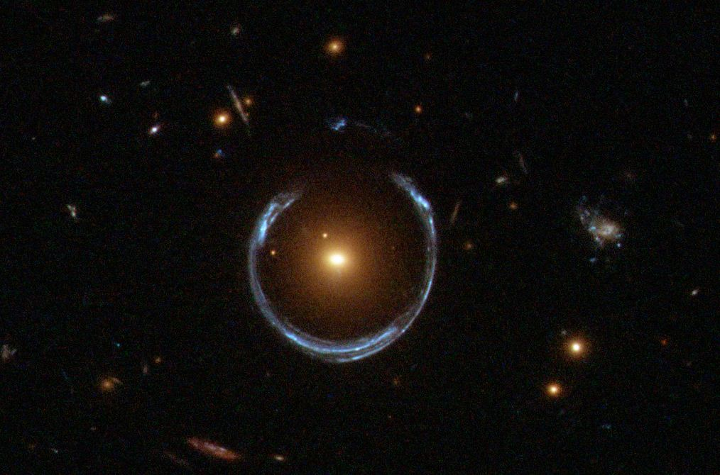
Gravitational Lensing

Einstein’s theory of General Relativity predicts that massive objects can bend the path of light. This effect is known as gravitational lensing. A gravitational lens is matter that bends light from a distant source as it travels towards an observer. This can be a star, black hole, galaxy, or even a cluster of galaxies.

Gravitational lensing can be categorized into three main types:

• Strong lensing is when there are easily visible distortions, such as the formation of Einstein rings, arcs, or multiple images of the same source.
• Weak lensing does not produce arcs or multiple images, but only flattens the shape of the source.
• Microlensing is when no distortion in shape can be seen, but the amount of light received from a background object changes.

The impact parameter $\xi$ is the shortest separation between the center of the lens and the path of a particular light ray. Here, L is the massive object (lens) at a distance $D_L$ from the observer, which bends the light emitted from the source S at a distance $D_S$. The observed images are S$_1$ and S$_2$. Angles $\theta$, $\phi$, and $\beta$ are very small. The deflection is given by

where $M$ is the mass of the lens.

From the diagram, we have that $\xi = \theta D_L$, and

Since $\phi = \frac{4GM}{c^2} \frac{1}{\theta D_L}$,

When the source is perfectly aligned with the lens ($\beta = 0$), a ring-like image is formed, called the Einstein ring, having angular radius (called the Einstein radius)

An example of an Einstein ring formed by gravitational lensing.

Using $\theta_E$, equation (5.5.2) can be rewritten as

which gives two solutions for $\theta$, corresponding to the two images formed

A property of gravitational lensing is that the surface brightness of the images formed remains the same as that of the original object. Thus the apparent brightness of the image is directly proportional to its area. From this, we can find out the amplification $\mu$ of light due to gravitational lensing

Evaluating this, we get

Cosmic Distance Ladder

There are several methods to find distances to celestial objects. Closer objects (moons, planets, sun) require a different technique to find their distance than distant objects like quasars. The cosmic distance ladder is a succession of methods by which astronomers determine the distances to celestial objects. Each method is built on the previous one, allowing for a more accurate measurement of distance.

Trigonometric Parallax

This is based on the apparent yearly back and forth movement of stars in the sky, caused by the orbital motion of Earth. This can measure distances up to ~30pc.

Statistical Parallax

The sun moves through the LSR with a speed of 20 km/s. Combining the apparent proper motion with observed radial motion allows the estimation of distance to a star cluster. This has been used to find the distance to Hyades.

Main Sequence Fitting

If the distance to a cluster is known, its HR diagram can be plotted. Another cluster whose distance is to be determined can be plotted on the same HR diagram and compared to get the distance modulus.

Standard Candles

Standard candles are classes of objects that have a calibrated absolute magnitude $M_V$.

Type Ia supernova is a type of supernova that occurs in binary systems in which one of the stars is a white dwarf. It occurs when the white dwarf exceeds the Chandrasekhar limit. The peak absolute magnitude of every Type Ia supernova is the same, $M_V = -19.3$.

Cepheid variables display a unique property known as the period-luminosity relationship. All cepheids exhibit a linear relationship between their luminosity and period. Another class of stars, RR Lyrae, also exhibit this property. The absolute magnitude of RR Lyrae stars is $M_V = 0.6$.

Hubble’s Law

Edwin Hubble discovered that galaxies move away from us with velocities proportional to their separation, i.e. that the universe is expanding. In terms of the redshift $z = \Delta \lambda / \lambda$,

where $H_0 = 70 \pm 7$ km/s/Mpc is the Hubble constant, and $r$ is the distance to the galaxy.

Apparent Superluminal Motion

Superluminal motion is the apparently faster-than-light motion seen in some radio galaxies. Bursts of energy moving out along the relativistic jets emitted from these objects can have a proper motion that appears greater than the speed of light.

It occurs usually when the source itself is moving at relativistic speeds, in a direction close to the line of sight.

Superluminal motion is most often observed in two opposing jets emanating from the core of a star or black hole. In this case, one jet is moving away from and one towards the Earth. If Doppler shifts are observed in both sources, the velocity and the distance can be determined independently of other observations.

Consider at time $t_1$, the source is at $A$ and at time $t_2 = t_1 + \delta t$ it moves to $B$. Then the photons emitted at $A$ at time $t_1$ are detected by the observer at

where $D_L$ is the distance from the source to the observer.

Photons emitted at $B$ at time $t_2$ are detected at

where $v \delta t \ll D_L$. Therefore the time difference between the two photons is

where $\beta = v/c$. The angle $\theta$ is the angle between the line of sight and the direction of motion of the source.

During the time $\Delta t$, the radio source will move by an angle $\Delta \phi$. Hence the proper motion $\mu$ is

This gives the transverse velocity

The maximum value of $\beta_t$ for a given $\beta$ occurs when $\theta = \cos^{-1} \beta$.

If $\gamma \gg 1$ (i.e. when velocity of jet is close to the velocity of light) then $\beta_t^\text{max} > 1$, means that the apparent transverse velocity along CB is larger than the velocity of light in vacuum, i.e. the motion is apparently superluminal.

Recombination and Decoupling

Recombination refers to the process in which free electrons combine with protons to form neutral hydrogen atoms. The epoch of recombination is the time at which the baryonic component of the universe goes from being ionized to neutral.

Decoupling refers to the process by which photons cease to interact significantly with matter. The epoch of photon decoupling is the time at which the rate at which the photons scatter from electrons becomes less than the Hubble parameter. This is when the universe becomes transparent to light. The epoch of last scattering is the time at which a typical CMB photon underwent its last scattering from an electron.

In the early universe, atoms and ions were in statistical equilibrium with each other

while the photons are still coupled to the baryonic component. In statistical equilibrium at temperature $T$, the number density $n_X$ of particles with mass $m_X$ is given by the Boltzmann distribution

when $kT \ll m_X c^2$. Here $g_X$ is the statistical weight of the particle $X$. For electrons, protons, and neutrons, $g = 2$. For Hydrogen, $g_H = g_p g_e = 4$.

Since $m_H \approx m_p$ and defining $Q = (m_p + m_e - m_H)c^2 \approx 13.6 \, \mathrm{eV}$ as the ionization energy, we have

This is called the Saha equation.

We define the fraction ionization $X$ as

From this we get that $n_H = \frac{1-X}{X} n_p$. For overall charge neutrality, we have $n_e = n_p$. Therefore

The ratio of baryonic number density and photon number density is

For a blackbody spectrum, $n_\gamma = 0.243 \left( \frac{kT}{\hbar c} \right)^3$.

For $X = 0.5$ and $\eta = 5.5 \times 10^{-10}$, we get $T_\text{rec} = 3740 \, \mathrm{K}$ and $z_\text{rec} = 1370$, which is $t = 240,000 \, \mathrm{yrs}$ after big bang.

The rate of photon scattering is

where $\sigma_e$ is the Thomson cross-section. Since $\frac{H^2}{H_0^2} = \Omega_{\text{m},0} (1+z)^3$, we get

The redshift of photon decoupling was found to be $z_\text{dec} = 1120$. However, the exact value is somewhat smaller, about $z_\text{dec} = 1090$, for which $T_\text{dec} = 2970 \, \mathrm{K}$ and $t = 371,000 \, \mathrm{yrs}$. The last scattering happened too around this time, $z_\text{ls} \approx z_\text{dec} \approx 1100$.