Three Body Systems

Guide

Three Body Systems

We now move on to the three body problem. Given the state of the system initially (i.e the positions and velocities of three point masses) orbiting each other in space, we wish to calculate the subsequent trajectory using newton’s laws of motion and gravitation. As it turns out, this is a much harder task than the two body problems, and a closed form solution doesn’t really exist.

When three bodies orbit each other, the resulting dynamical system is chaotic for most initial conditions. Because there are no solvable equations for most three-body systems, the only way to predict the motions of the bodies is to estimate them using numerical methods.

However, there is still some analysis we can do. In particular, there are a class of problems called the restricted three body problems, which are much easier to analyze theoretically. Two massive bodies, called primaries, orbit each other in a circular orbit, and a third body of negligible mass moves under the influence of the two massive bodies. The third body does not affect the motion of the two massive bodies.

Anyway, there do exist some special configurations, for which solutions to the three body problem are known. Two of them are:

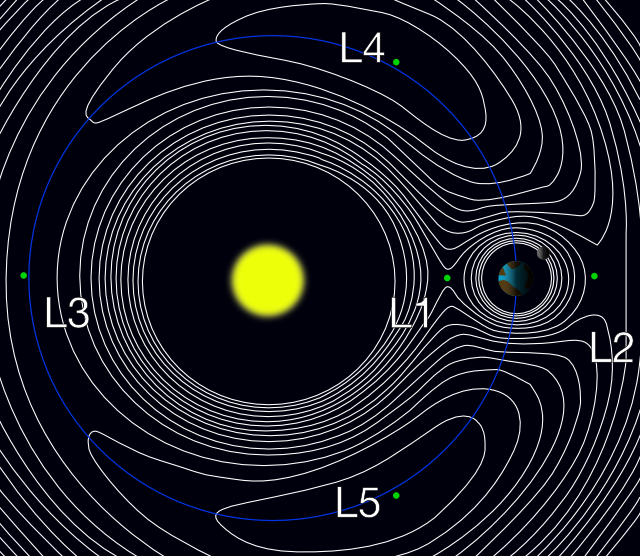
Lagrange points: This is a solution to the restricted three body problem. Five points exist in the orbital plane of two massive bodies, where a third body can be placed and remain in a stable position relative to the two massive bodies. The Lagrange points are denoted $L_1$ , $L_2$ , $L_3$ , $L_4$ , and $L_5$ . The $L_4$ and $L_5$ points are stable, while the others are unstable.
8 shaped orbit: This is a solution to the full three body problem. Three bodies of equal masses can orbit each other in a figure-eight pattern. This solution is known as the Chenciner–Montgomery orbit. The total angular momentum of such a system is zero, and the three bodies lie in a plane.

Virial Theorem

One very important theorem, that has is useful even beyond astrophysics is the virial theorem. Suppose we have a system of $n$ point masses $m_i$ with position vectors $\mathbf{r}_i$ and velocities $\mathbf{v}_i$ , where the only force of consideration is gravity.

For the theorem to hold, we make two assumptions about our system:

The time averages of the total kinetic energy and the total potential energy are well-defined.
The velocities and positions of all particles are bounded (they don’t shoot off to infinity).

The time average of $\xi$ over some time interval $[0, \tau]$ , denoted as $\lang \xi \rang$ , is:

\lang \xi \rang = \frac{1}{\tau} \int_0^\tau \xi(t)\; dt

It is worth thinking about this definition for a moment.

The virial theorem then states that over a large time period, we have:

\tag{3.5.1} \boxed{2 \, \lang K \rang + \lang U \rang = 0 }

where $K$ and $U$ are the kinetic and (gravitational) potential energies of the system, respectively.

The theorem is quite magical in nature, you get a relation between kinetic and potential energies out of nowhere! Just for a sanity check, noting that the assumptions work for the case of a closed two body system (for example, one with a circular orbit), let’s try to check if this result holds true.

Consider the case of a light particle of mass $m$ orbiting a heavy one $M$ in a circular orbit (in particular, the velocity of the heavy particle is near zero and thus is its kinetic energy, because $M \gg m$ ). The potential energy is simply $-GmM/r$ where $r$ is the radius of the orbit. For the kinetic energy, note that the gravitational force acting on the smaller mass is the centripetal force, so that ${mv^2}/{r} = GmM/r^2 \implies v^2 = GM/r$ , so that $K = GMm/2r$ , thus $2 \, \lang K \rang + \lang U \rang = 0$ as expected!

Now let’s prove the theorem. We define the virial of the system, $A$ as:

\tag{3.5.2} A = \sum_{i=1}^n m_i \mathbf{v}_i \cdot \mathbf{r}_i = \sum_{i = 1}^n \mathbf{p}_i \cdot \mathbf{r}_i

\implies \dot{A} = 2\,K + \sum_{i=1}^n \mathbf{F}_i \cdot \mathbf{r}_i

where $K$ is the total kinetic energy of the system, and $F_i$ is the force on the $i$ th body. Let $\lang x \rang$ denote the time average of $x$ in the interval $[0, \tau]$

\lang \dot{A} \rang = \frac{1}{\tau} \int_0^\tau \dot{A} dt = \frac{A(\tau) - A(0)}{\tau} = 2\, \lang K \rang + \lang \sum_{i=1}^n \mathbf{F}_i \cdot \mathbf{r}_i\rang

By our first assumption, the time averages of the kinetic and potential energy are well defined so the equality holds. By our second assumption, $A$ remains finite, so as $\tau \rightarrow \infty$ , $\{A(\tau) - A(0)\}/{\tau} \rightarrow 0$ . For gravitational forces, $\sum_{i=1}^n \mathbf{F}_i \cdot \mathbf{r}_i = U$ , hence we get that $2 \lang K \rang + \lang U \rang = 0$ .

Although the theorem is only true for bounded systems, it is often the case that in astrophysics our system is not bounded. For example, a galaxy will occasionally fling stars into the vastness of space, making their position unbounded as a function of time. This process of “boiling off” is very important in the long run. But it’s very slow, so the conditions of the virial theorem seem to be “approximately true” in the short run.

Most people go ahead and use it without worrying about this subtlety. To justify this, we should modify the above argument by averaging not over an infinite time, but a finite time. This time should be long compared to the time it takes stars to go around the galaxy, while still short compared to the time it takes for them to boil off. Then we’ll approximately get $2 \, \lang K \rang + \lang U \rang = 0$ .

🧮

General Virial Theorem

You can extend the theorem to systems with potential energy $U$ of the form $\alpha r^n$ , where $r$ is the distance between two bodies. This is of course, the potential energy of a central force, $\mathbf{F} = n\alpha r^{n-1} \mathbf{\hat{r}}$ . We also swept the calculation of $\sum_{i=1}^n \mathbf{F}_i \cdot \mathbf{r}_i = U$ under the rug, which we’ll deal with in general now.

We assume there are no external forces on the system. Then, the force on a single particle $\mathbf{F}_k$ is the sum of forces due to all the particles,

\mathbf{F}_k = \sum_{j=1}^{N} \mathbf{F}_{jk}

where $\mathbf{F}_{jk}$ is the force applied by particle $j$ on particle $k$ . The diagonal term $F_{kk}$ term here is just $0$ (because a particle can’t apply a force on itself), so we split the sum into upper and lower terms:

{\begin{aligned}\sum _{k=1}^{N}\mathbf {F} _{k}\cdot \mathbf {r} _{k}&=\sum _{k=1}^{N}\sum _{j=1}^{N}\mathbf {F} _{jk}\cdot \mathbf {r} _{k}=\sum _{k=2}^{N}\sum _{j=1}^{k-1}\mathbf {F} _{jk}\cdot \mathbf {r} _{k}+\sum _{k=1}^{N-1}\sum _{j=k+1}^{N}\mathbf {F} _{jk}\cdot \mathbf {r} _{k}\\&=\sum _{k=2}^{N}\sum _{j=1}^{k-1}\mathbf {F} _{jk}\cdot \mathbf {r} _{k}+\sum _{j=2}^{N}\sum _{k=1}^{j-1}\mathbf {F} _{jk}\cdot \mathbf {r} _{k}=\sum _{k=2}^{N}\sum _{j=1}^{k-1}(\mathbf {F} _{jk}\cdot \mathbf {r} _{k}+\mathbf {F} _{kj}\cdot \mathbf {r} _{j})\\&=\sum _{k=2}^{N}\sum _{j=1}^{k-1}(\mathbf {F} _{jk}\cdot \mathbf {r} _{k}-\mathbf {F} _{jk}\cdot \mathbf {r} _{j})=\sum _{k=2}^{N}\sum _{j=1}^{k-1}\mathbf {F} _{jk}\cdot (\mathbf {r} _{k}-\mathbf {r} _{j}),\end{aligned}}

where $\mathbf{F}_{kj} = -\mathbf{F}_{jk}$ by newton’s third law.

Now $\mathbf{F}_{jk}$ is related to the potential energy as:

\mathbf{F}_{jk} = -\frac{dU_{jk}}{dr_k} = -\frac{dU_{jk}}{dr_{jk}} \left(\frac{\mathbf{r}_k - \mathbf{r}_j}{r_{jk}}\right)

by the chain rule.

Thus,

{\displaystyle {\begin{aligned}\sum _{k=1}^{N}\mathbf {F} _{k}\cdot \mathbf {r} _{k}&=\sum _{k=2}^{N}\sum _{j=1}^{k-1}\mathbf {F} _{jk}\cdot (\mathbf {r} _{k}-\mathbf {r} _{j})\\&=-\sum _{k=2}^{N}\sum _{j=1}^{k-1}{\frac {dU _{jk}}{dr_{jk}}}{\frac {|\mathbf {r} _{k}-\mathbf {r} _{j}|^{2}}{r_{jk}}}\\&=-\sum _{k=2}^{N}\sum _{j=1}^{k-1}{\frac {dU_{jk}}{dr_{jk}}}r_{jk}.\end{aligned}}}

For the power law potential, $dU_{jk}/dr_{jk} = nU_{jk}$ , thus,

{\begin{aligned}-{\frac {1}{2}}\,\sum _{k=1}^{N}\mathbf {F} _{k}\cdot \mathbf {r} _{k}&={\frac {1}{2}}\,\sum _{k=1}^{N}\sum _{j<k}{\frac {dU_{jk}}{dr_{jk}}}r_{jk}\\&={\frac {1}{2}}\,\sum _{k=1}^{N}\sum _{j<k}n\alpha r_{jk}^{n-1}r_{jk}\\&={\frac {1}{2}}\,\sum _{k=1}^{N}\sum _{j<k}nU_{jk}={\frac {n}{2}}\,U_{\text{TOT}},\end{aligned}}

where $U_{TOT}$ is the total potential energy of the system. Dropping the subscript, we finally get that,

\lang T \rang = \frac{n}{2} \lang U \rang

using our previous derivation.

Hill Sphere

The Hill sphere is the region around a celestial body where its own gravity (compared to other nearby bodies) is the dominant force in attracting satellites. It is also known as the Roche sphere. If a less massive body $m$ orbits a (more) massive body $M$ ( $M \ll m$ ), and has an instantaneous distance $a$ from $M$ , then its hill radius (at that instant) is

\tag{3.5.3} \boxed{ R_H \approx a \left( \frac{m}{3(M + m)} \right)^{1/3} }

For Earth, this is approximately $0.01 \mathrm{\,AU}$ . The derivation of the hill radius is similar to that of the $L_1$ and $L_2$ Lagrange points.

Lagrange Points

In the restricted three body problem, the third body can remain at rest relative to the primaries at certain points. When seen in a rotating reference frame, a body kept at one of the Lagrange points matches the angular velocity of the two co-orbiting primaries, allowing it to remain stationary relative to them. At the Lagrange points, the net gravitational force acting on the third body is equal to the centrifugal force acting on it.

This is a particular configuration which can be solved, that is to say we can predict the subsequent motion of the bodies. Since the third body is at rest, we only need to worry about the other two bodies, because its mass is much lower, and so doesn’t affect the other two bodies much.

There are five such points, called Lagrange points. The Lagrange points are denoted $L_1$ , $L_2$ , $L_3$ , $L_4$ , and $L_5$ . The points $L_1$ , $L_2$ and $L_3$ are unstable, and lie on the line joining the two primaries. The points $L_4$ and $L_5$ are stable (well, not exactly, but we’ll talk about this in a second) and lie at the vertices of equilateral triangles with the two primaries (the more massive bodies).

We will refer to something called the barycenter in the following discussion, which is defined to be center of mass of the three-body system, and is also the center of rotation of the three-body system.

The Lagrange points are positions in space where the gravitational forces of two large bodies balance the centripetal force felt by a smaller object. (Source: Wikipedia)

Asteroids and comets are often found at the Lagrange points of the Sun and Jupiter. The Lagrange points are also used for placing satellites in orbit. Asteroids found around Jupiter’s $L_4$ and $L_5$ points are called Trojan asteroids.

Let the masses of the two primaries be $M$ and $m$ ( $M > m$ ), separated at a distance $R$ . Consider the co-ordinate system with the centre of mass as the centre. Since the mass of the third body is negligible, the centre of mass is the same as the centre of mass of $M$ , and $m$ .

You might remember from bound orbits that the angular velocities of the two bodies about the centre of mass are same. We’ll quickly show this again. Since the centripetal force is gravity, we get that,

M\omega^2 r_1 = \frac{GmM}{R^2}

where $r_1$ is the distance of $M$ from the centre. Since the centre is the centre of mass, we get that $m/r_1 = (M + m)/R$ which gives us the angular velocity for the body, as:

\tag{3.5.4} \omega = \sqrt{ \frac{G(M + m)}{R^3} }

A similar derivation for the other primary will give you the same angular velocity.

L ₁

The $L_1$ point lies between the two primaries, and its distance $r$ from the small primary is given by

\tag{3.5.5} \frac{GM}{(R-r)^2} - \frac{Gm}{r^2} = \left( \frac{m}{M + m} R - r \right) \omega^2

by balancing centrifugal forces, and noting that the term on the right hand in parentheses the distance of $L_1$ from centre of mass. This turns out to be a quintic on expanding. Analytic solutions are as such not possible, but we can find $L_1$ using numerical methods.

If $M \gg m$ , then $L_1$ and $L_2$ are approximately at the same distance $r$ from the smaller primary, equal to the hill radius, given by

\tag{3.5.6} r \approx R \sqrt[3]{\frac{m}{M+m}}

L ₂

The $L_2$ point lies on the opposite side of the larger primary, and its distance $r$ from the smaller primary is given by

\tag{3.5.7} \frac{GM}{(R+r)^2} + \frac{Gm}{r^2} = \left( \frac{m}{M + m} R + r \right) \omega^2

Again, if $M \gg m$ , then $L_1$ and $L_2$ are approximately at the same distance $r$ from the smaller primary, equal to the hill radius, given by

\tag{3.5.8} r \approx R \sqrt[3]{\frac{m}{M+m}}

We can also write this relation as

\frac{m}{r^3} \approx \frac{M}{R^3}

Now, since $F_\text{tidal} \propto {M}/{R^3}$ , we find that the tidal effect of the smaller primary at the $L_1$ or at the $L_2$ point is about three times of that the larger primary. We can also write the relation as

\rho_2 \alpha_2^3 \approx 3 \rho_1 \alpha_1^3

where $\rho$ is the density of the primary and $\alpha$ is its angular size, as seen from $L_1$ or $L_2$ . This shows that viewed from these two Lagrange points, the apparent sizes of the two bodies will be similar, especially if the density of the smaller one is about thrice that of the larger, as in the case of the earth and the sun. Looking toward the sun from $L_2$ one sees an annular eclipse. Therefore it is necessary for a spacecraft parked at $L_2$ , to follow a Lissajous orbit or a halo orbit around $L_2$ in order for its solar panels to get full sun.

L ₃

The $L_3$ point lies on the opposite side of the smaller primary, and its distance $r$ from the orbit of the smaller primary is given by

\tag{3.5.9} \frac{GM}{(R-r)^2} + \frac{Gm}{(2R-r)^2} = \left( \frac{m}{M + m} R + R - r \right) \omega^2

If $M \gg m$ , then

\tag{3.5.10} r \approx \frac{7}{12}\frac{m}{M+m}R

L ₄ and L ₅

The reason these points are in balance is that $L_4$ , $L_5$ are the third vertices of equilateral triangles with the two primaries as other two vertices. What this causes is that the forces are proportional to the masses, and so the resultant on all bodies acts through the line from the barycenter (centre of mass) to the body. The angular velocities due to the resultant, centripetal force are equal.

In fact, in general, if you’ve a (non-degenerate) triangle $\Delta ABC$ , where there are three masses at the vertices, the only way to have the system rotate as a rigid body around the barycenter is to have ot be an equilateral triangle. The sketch of the proof is as such:

Clearly, the three masses move with the same angular velocity because it rotates as a rigid body. And since the body rotates around as a rigid body, the distances between the masses do not change, so the gravitational potential energy is unchanged. Since the system is isolated, there are no external forces on it and the total energy is conserved. Accordingly, the kinetic energy must be conserved as well. Then, since the moment of inertia is just $m_ir_i^2$ about the barycenter, where $r_i$ is the distance of $m_i$ from the barycenter, and distances remain unchanged, and the kinetic energy about the barycenter $\sum I_i\omega^2$ is also unchanged, $\omega$ must be the same throughout the motion as well.

Great, now for the body to be at rest in the frame rotating with angular speed $\omega$ , the gravitation forces must balance the centrifugal force. Let the distance between masses $m_i$ , $m_j$ be $a_{ij}$ . Using a co-ordinate system with the barycenter as the centre, the position vector of mass $m_i$ is denoted $\mathbf{r}_i$ . Because we are working in the centre of mass frame, $m_1\mathbf{r}_1 + m_2\mathbf{r}_2+ m_3\mathbf{r}_3 = 0$ . By force balance on $m_1$ :

\begin{aligned} &\frac{Gm_1m_2}{a_{12}^3} (\mathbf{r}_2 - \mathbf{r}_1) + \frac{Gm_3m_1}{a_{13}^3} (\mathbf{r}_3 - \mathbf{r}_1) + m_1\omega^2\mathbf{r}_1 = 0 \\ &\implies \frac{Gm_2}{a_{12}^3} (\mathbf{r}_2 - \mathbf{r}_1) + \frac{Gm_3}{a_{13}^3} (\mathbf{r}_3 - \mathbf{r}_1) = -\omega^2\mathbf{r}_1 \\ &\implies \frac{Gm_2}{a_{12}^3} \mathbf{r}_2 + \frac{Gm_3}{a_{13}^3} \mathbf{r}_3 = \mathbf{r}_1\left( \frac{Gm_2}{a_{12}^3} + \frac{Gm_3}{a_{13}^3} - \omega^2\right) \\ \end{aligned}

Now, by using $m_1\mathbf{r}_1 + m_2\mathbf{r}_i+ m_3\mathbf{r}_3 = 0 \implies m_2\mathbf{r}_2 = -(m_1\mathbf{r}_1+ m_3\mathbf{r}_3)$ , we get that:

{Gm_3}\mathbf{r}_3\left(\frac{1}{a_{13}^3} - \frac{1}{a_{12}^3}\right) = \mathbf{r}_1\left( \frac{Gm_2 + Gm_1}{a_{12}^3} + \frac{Gm_3}{a_{13}^3} - \omega^2\right)

Since the triangle is not degenerate, $\mathbf{r}_1 \nparallel \mathbf{r}_3$ , so the coefficients must be zero. Subsequently, you get that $a_{12} = a_{13} = a$ . Repeating this for all the three masses, you get that the triangle is equilateral, and that $\omega = \sqrt{G(m_1 + m_2 + m_3)/a^3}$ .

As it turns out, for certain configurations, $L_4$ and $L_5$ points are stable. This is especially helpful, as satellites can correct their orbit if perturbed easily (remember that for stable points, the force points towards that point, so that the body is pulled back in the case of small displacements, as opposed to push away— when the point is unstable). The condition for stability is that the ratio of the masses of the two primaries must exceed $25(1/2 + \sqrt{1/4 - 1/625})$ . I will not prove this here, as it takes quite a bit of work, but you can read this article by Jaan Kalda for a thorough treatment of the problem

Orbital Resonance

Orbital resonance occurs when orbiting bodies exert regular, periodic gravitational influence on each other, usually because their orbital periods are related by a ratio of small integers. Examples are the 1:2:4 resonance of Jupiter’s moons Ganymede, Europa and Io, and the 2:3 resonance between Neptune and Pluto. Unstable resonances with Saturn’s inner moons give rise to gaps in the rings of Saturn. The special case of 1:1 resonance between bodies with similar orbital radii causes large planetary system bodies to eject most other bodies sharing their orbits; this is part of the much more extensive process of clearing the neighbourhood around planets.

A binary resonance ratio should be interpreted as the ratio of number of orbits completed in the same time interval, rather than as the ratio of orbital periods, which would be the inverse ratio. Thus, the 2:3 ratio above means that Pluto completes two orbits in the time it takes Neptune to complete three.

A mean-motion orbital resonance occurs when two bodies have periods of revolution that are a simple integer ratio of each other.

A spin orbit resonance is where the spin period of the planet is connected to the orbital period by a simple ratio. For circular orbits, only such resonance possible is 1:1, where the planet is tidally locked to the star. For elliptical orbits, other resonances are possible. Mercury has a spin orbit resonance or 3:2 with the sun, where it rotates three times on its axis for every two revolutions around the sun.

n-body problem

The n-body problem is the problem of predicting the individual motions of a group of celestial objects interacting with each other gravitationally. It consists of n point mass $m_i$ , with position vectors $\mathbf{r}_i$ and velocities $\mathbf{v}_i$ . The equations of motion are given by

\tag{3.5.11} \ddot{\mathbf{r}}_i = \sum_{\substack{j=0 \\ j \neq i}}^{n} \frac{G m_i m_j}{|\mathbf{r}_j - \mathbf{r}_j|^3} (\mathbf{r}_j - \mathbf{r}_i)

There is no general closed form solution for $n >2$ .

Problems

Find the first cosmic velocity, which is the least velocity of a satellite launched from the surface of Earth required to put a satellite into orbit around the earth.

The first cosmic velocity is given by

\tag{3.5.11} v_1 = \sqrt{\frac{GM_\oplus}{R_\oplus}} \approx \boxed{7.91 \mathrm{\,km/s}}

Find the second cosmic velocity, which is the least velocity of a satellite launched from the surface of Earth required to escape from the gravitational field of the earth.

The second cosmic velocity is given by

\tag{3.5.12} v_2 = \sqrt{\frac{2GM_\oplus}{R_\oplus}} \approx \boxed{11.2 \mathrm{\,km/s}}

Find the third cosmic velocity, which is the least velocity of a satellite launched from the surface of Earth required to escape from the gravitational field of the solar system.

In heliocentric frame, the escape velocity is

v_{2,\odot} = \sqrt{\frac{2GM_\odot}{a_\odot}} \approx 42.1 \mathrm{\,km/s}

From Earth’s frame,

v' = v_{2,\odot} - v_\oplus = \sqrt{\frac{2GM_\odot}{a_\odot}} - \sqrt{\frac{GM_\odot}{a_\odot}} \approx 12.3 \mathrm{\,km/s}

Therefore, we can get the third cosmic velocity by

\frac{1}{2} v_3^2 - \frac{GM_\oplus}{R_\oplus} = \frac{1}{2}v'^3

\tag{3.5.13} \implies v_3 = \sqrt{\frac{2GM_\oplus}{R_\oplus} + v'^2} \approx \boxed{16.7 \mathrm{\,km/s}}

Estimate the number of stars in a globular cluster of diameter 40 pc, if the escape velocity at the edge of the cluster is 6 km/s and most of the stars are similar to the Sun.

The escape velocity of object on the edge of the cluster is given by

v_e = \sqrt{ \frac{2GM}{R} } \implies M = \frac{Rv_e^2}{2G}

N = \frac{M}{M_\odot} = \frac{Rv_e^2}{2GM_\odot} \approx \boxed{ 8.4 \times 10^4 }

Orbital Elements Orbital Maneuvers

Three Body Systems

Virial Theorem

Hill Sphere

Lagrange Points

L 1

L 2

L 3

L 4 and L 5

Orbital Resonance

n-body problem

Problems

L ₁

L ₂

L ₃

L ₄ and L ₅